Multiple CTEs in a Query

The following is chapter 6 from my Common Table Expressions book in its entirety.

READER NOTE: Please run the CTEBookSetup.sql script in order to follow along with the examples in this chapter. The script mentioned in this chapter is available at http://SteveStedman.com.

Thinking of the proverb “two heads are better than one” makes me think, it really depends on the people. Two people working together are indeed better than one if they can work together and have the same goals. If there are two people who don’t work well together then perhaps the proverb is not true.

With CTEs the proverb may be “two CTEs are better than one, when it makes sense” meaning that there are times you can accomplish exactly what you want to accomplish with a single CTE, but there are times that you could do it quicker or easier with multiple CTEs. Some of the same reasons that you might work with a CTE to begin with could be used to determine when it is appropriate to use multiple CTEs.

There are several different things that can be done with multiple CTEs in a single query. If it makes sense to break out one derived table into a CTE it may make sense to break out two. With multiple CTEs in the same query, later CTEs can access the earlier CTEs; this is called a nested CTE. Just as a SELECT statement can access multiple tables it can also access multiple CTEs in the same statement.

READER NOTE: Please run the CTEBookSetup.sql script in order to follow along with the examples in this chapter. The script mentioned in this chapter is available at http://SteveStedman.com.

Adding a Second CTE

The same steps for adding a second CTE can be repeated to add a third, fourth, or more CTE queries.

The steps to add a second CTE into a query are:

Add a comma at the end of the first CTE, after the closing parentheses.
After the comma, on the next line, declare the name of the new CTE.
After the name of the new CTE add the optional columns declaration.
Add the AS keyword followed by opening and closing parentheses.
Inside of the parentheses add the new CTE query.
Call the CTE query from the outer SELECT statement.

Before we can add a second CTE we need a query that uses a single CTE that it can be added to. To start with we will use a single CTE that simply displays three names from the CTE. This is not a recursive query, but it is using the UNION set operator to place the three names into the result set.

;WITH Fnames (Name) AS
(
SELECT ‘John’
UNION
SELECT ‘Mary’
UNION
SELECT ‘Bill’
)
SELECT F.Name AS FirstName
FROM Fnames F;

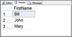
Figure 6.1 Output from the Fnames CTE query.

The query in the previous example selects a number of first names as a result set. It could have been expanded upon to have hundreds of first names, but for the purpose in this example we will keep the list small.

To add the second CTE follow the steps outlined earlier. Add a comma after the first CTE, name the second CTE and declare the columns. Add the AS keyword, parentheses, the CTE query, and then access it from the outer SELECT statement.

In the following example, we will be adding a series of last names into the first names list from the previous CTE. For the list of last names the same UNION style query of three results will be used to build a result of three last names.

SELECT ‘Smith’
UNION
SELECT ‘Gibb’
UNION
SELECT ‘Jones’;

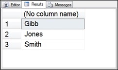
Figure 6.2 Output of the three unioned SELECT statements.

Now place the Lnames CTE into the existing query as seen in the following code:

;WITH Fnames (Name) AS
(
SELECT ‘John’
UNION
SELECT ‘Mary’
UNION
SELECT ‘Bill’
),
Lnames (Name) AS
(
SELECT ‘Smith’
UNION
SELECT ‘Gibb’
UNION
SELECT ‘Jones’
)
SELECT F.Name AS FirstName, L.Name AS LastName
FROM Fnames AS F
CROSS JOIN Lnames AS L;

The previous example uses a CROSS JOIN which creates a Cartesian product of the two inputs. This matches up every element from Fnames with every element from Lnames producing a total of three times three (or 9) rows in the result set.

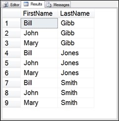
Figure 6.3 Output from Fnames CTE cross joined with the Lnames CTE.

The previous example works great in SQL Server 2005 and newer. In SQL Server 2008 there was a new feature called “row constructors” introduced that can simplify the overall syntax of a CTE query like we are using here. It has nothing to do with the CTE, it just simplifies the query inside the CTE.

With the row constructor we can replace the inner union queries, for instance:

SELECT ‘Smith’
UNION
SELECT ‘Gibb’
UNION
SELECT ‘Jones’;

Is replaced with:

SELECT x FROM (VALUES (‘Smith’), (‘Gibb’), (‘Jones’)) f(x);

Which simplifies the following query:

;WITH Fnames (Name) AS
(
SELECT x FROM (VALUES (‘John’), (‘Mary’), (‘Bill’)) f(x)
),
Lnames (Name) AS
(
SELECT x FROM (VALUES (‘Smith’), (‘Gibb’), (‘Jones’)) f(x)
)
SELECT F.Name AS FirstName, L.Name AS LastName
FROM Fnames F
CROSS JOIN Lnames as L;

Figure 6.4 Same result from the simplified CTE query as the original.

In the previous examples there were no tables involved, however the exact same syntax that was used to build these queries could be done with tables.

When using multiple CTEs in a single query, those CTEs can be comprised of a single anchor query, multiple anchor queries, no recursive query, a single recursive query or multiple recursive queries. Any of the things that can be done with a single CTE can be done with each of the single CTEs in a multiple CTE query. There are things that can only be done with multiple CTEs such as the concept of nesting CTEs.

Nesting CTEs

If you have ever seen the Matryoshka dolls known as the Russian nesting dolls or babushka dolls they are very interesting. They start with a large wooden doll that when opened contains a slightly smaller doll, then inside of that one an even smaller doll. These dolls often have five to eight dolls nested inside of each other.

The interesting thing about these dolls is that they have one specific way that they can all fit together; the smallest doll must be the first one put inside of the next smallest. If you were to lose one of the medium dolls, they could still be placed together; there would just be some extra space inside.

Nested CTEs often remind me of the Russian nesting dolls. Think of the first CTE in a multiple CTE query as the smallest doll. That first CTE can’t reference any other CTEs, much like the smallest doll can’t fit any other dolls inside of it.

Think of the second CTE in a multiple CTE query as the second smallest doll in the Russian dolls. It can only have one doll fit inside of it. CTEs are similar in that the only CTE that can be referenced by the second CTE in a multiple CTE query is the first CTE.

The third CTE is like the third smallest Russian doll. The third smallest doll can only have the smallest or second smallest doll placed inside of it. With the third CTE it can only access the first or the second CTE declared, and not any of the CTEs declared later.

The same concept applies for all of the CTEs in a nested CTE query. Any CTE query can access the CTEs declared prior to that one, but not the ones after.

This is the scope of the CTE. In the introduction to CTEs section of this book we learned that the scope of a CTE is only a single query. This is narrowed down a bit farther, in that the scope of a CTE is only a single query, but only that part of the query declared after that CTE.

Take an example of a multiple CTE query with 4 CTEs as follows with the … being replaced with a T-SQL query.

;WITH CTE1 AS
( …. ),

CTE2 AS
( …. ),

CTE3 AS
( …. ),

CTE4 AS
( …. )

SELECT *
FROM CTE4;

The following diagram represents what each part of the CTE query has access to. Any CTE can access that which is contained in the box with its name. The outer query can use any of the CTEs. CTE4 has access to CTE1 to CTE3, and technically CTE4 if it is a recursive CTE. The things that CTE3 can’t access are CTE4 and the outer query. CTE2 only has access to itself and to CTE1, and CTE1 in this example can’t access any of the other CTEs in the query.

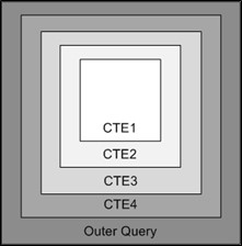
Figure 6.5 Scope diagram for nested CTEs.

Let’s say we wanted to query the JProCo database to find the top 10 customers with the most orders. We need to display their name and we want to look up the number of ordered items for each of the customers. As with most any request like this there are many different ways to do it. It could be done with a large query with several derived tables, or it could be done with multiple nested CTEs.

We can begin by building a CTE to get the top 10 customers by number of orders. It could look like this:

;WITH CustomersWithMostOrdersCTE AS
— First CTE
(
  SELECT TOP 10 CustomerID, count(1) AS numOrders
    FROM SalesInvoice
   GROUP BY CustomerID
   ORDER BY count(1) desc
)
SELECT *
FROM CustomersWithMostOrdersCTE;

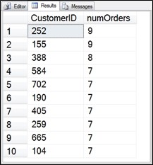
Figure 6.6 CustomersWithMostOrdersCTE output.

Once we have the customers with the most orders, another CTE can be added to add the customer names into the results. Now technically, this could be done in many other ways without a nested CTE, but keep in mind the nested CTE works just as well as other methods.

Notice that in the following query the first CTE is referenced from the second CTE, and only inside of the second CTE. If the need arises, there is no reason that the first CTE couldn’t have been accessed from both the second CTE, and the outer query.

;WITH CustomersWithMostOrdersCTE AS
— First CTE
(
  SELECT TOP 10 CustomerID,
                count(1) as numOrders
    FROM SalesInvoice
   GROUP BY CustomerID
   ORDER BY count(1) DESC
),
— Second CTE
CustomersOrdersWithNamesCTE AS
(
  SELECT cust.FirstName, cust.LastName,
         cte.*
    FROM Customer AS cust
   INNER JOIN CustomersWithMostOrdersCTE AS cte
           ON cte.CustomerID = cust.CustomerID
)
SELECT *
FROM CustomersOrdersWithNamesCTE;

This gives us the same 10 customers as the previous query but there are more columns included in the output.

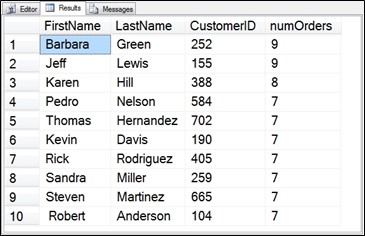
Figure 6.7 Output from the nested CTE called CustomersOrdersWithNamesCTE.

At this point the CTEs would be considered nested since one CTE references the other.

Now we will add another CTE to get the total number of items per invoice. This CTE will not be nested, as it will only be accessed from the outside query, and not from inside of any CTE, and it is does not reference any of the other CTEs.

;WITH CustomersWithMostOrdersCTE AS
— First CTE
(
  SELECT TOP 10 CustomerID,
                count(1) as numOrders
    FROM SalesInvoice
   GROUP BY CustomerID
   ORDER BY count(1) desc
),
— Second CTE
CustomersOrdersWithNamesCTE AS
(
  SELECT cust.FirstName, cust.LastName,
         cte.*
    FROM Customer AS cust
   INNER JOIN CustomersWithMostOrdersCTE AS cte
           ON cte.CustomerID = cust.CustomerID
),
— Third CTE
OrderItemsPerCustomerCTE AS
(
  SELECT  invoice.CustomerID, count(1) as numItems
    FROM SalesInvoice as invoice
   INNER JOIN SalesInvoiceDetail as detail
           ON detail.invoiceID = invoice.invoiceid
   GROUP BY invoice.CustomerID
)
SELECT FirstName, LastName,
       NumOrders, NumItems
FROM OrderItemsPerCustomerCTE AS items
INNER JOIN CustomersOrdersWithNamesCTE AS names
         ON items.CustomerID = names.CustomerID;

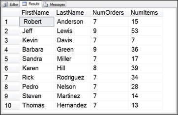
Figure 6.8 Output from three CTEs, two are nested, and the third is not.

To walk through what is happening with the example shown in Figure 6.8 follow these steps:

The outer SELECT statement is accessing OrderItemsPerCustomerCTE and CustomersOrdersWithNamesCTE.
CustomersOrdersWithNamesCTE references a table and it also references CustomersWithMostOrdersCTE which is considered nested.
CustomersWithMostOrdersCTE doesn’t reference any CTEs, it only references tables.
OrderItemsPerCustomerCTE doesn’t reference any CTEs, it also only references tables.

In this result we have ended up with 3 CTEs, two nested, and one not nested. If the need arises, we can have nested CTEs that are many levels deep.

Nesting CTEs can be a great way to accomplish queries that would otherwise have been difficult to create.

How Many Levels of Nesting

The question of how many levels of nesting are allowed is a dangerous one, and perhaps should be reworded as “How many levels should we nest CTEs?” The answer to the question of can versus should is that we should only nest what we need to nest. A few dozen or even up to 100 nested CTEs shouldn’t pose a problem. The number of nested levels you can use depends on the version of SQL Server being used.

SQL Server 2005 has a limit of 256 table names in a query. This 256 table name limit also applies to CTE names.

with cte0 as
(select 1 as num)
, cte1 AS (SELECT * FROM cte0)
, cte2 AS (SELECT * FROM cte1)

Repeated from 2 to 254

, cte255 AS (SELECT * FROM cte254)
, cte256 AS (SELECT * FROM cte255)
, cte257 AS (SELECT * FROM cte256)
select * from cte257;

In SQL Server 2005 the error shown in Figure 6.9 is thrown.

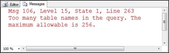
Figure 6.9 Output from query with multiple CTEs.

The previous example runs just fine if we trim one of the CTE references out of it.

For SQL Server 2008, 2008R2 and 2012, the nested CTE limit appears to be a limitation of the available memory. On a 2012 SQL Server with 8 GB of RAM, 1600 levels of CTE nesting works well. But if you try 1700 levels of nesting it fails with an insufficient memory error. On that same computer with an additional 16 GB of RAM added for a total of 24 GB, 2300 levels of CTE nesting works, but 2400 doesn’t.

Generally, SQL Server 2008 and newer will run out of memory before any built in maximum is hit. So the real answer to how many levels can be nested is “it depends”. It really depends on the amount of memory available.

The limits on levels of nesting are probably more than should ever be needed. It might be worth reassessing the logic before attempting to create a nested CTE more than a few hundred levels deep.

Additional Breakdown of Derived Tables

In Chapter 3 a derived table was covered, but multiple CTEs were not covered at that point, so the examples in chapter 3 only involve the use of a single CTE to help with cleaning up derived tables.

Everything that was covered as to why we should convert a derived table into a CTE still applies with multiple CTEs; those reasons are just more valuable. If it made sense to break out a single derived table query into a CTE, it makes sense to break out two, three or many derived tables into a CTE.

Take the following example which makes use of two different derived tables. They are similar, but not identical.

SELECT q1.department, q2.department as subDepartment
FROM (SELECT id, department, parent
          FROM Departments
         WHERE id = 4) as q1
INNER JOIN (SELECT id, department, parent
               FROM Departments) as q2
         ON q1.id = q2.parent;

Figure 6.10 Output from query with multiple derived tables.

The first derived table query looks like this:

SELECT id, department, parent
FROM Departments
WHERE id = 4

The second derived table query looks like this:

SELECT id, department, parent
FROM Departments

In chapter 3 the following steps were established as a way to break derived tables out into a CTE.

Find the first occurrence of the derived table query to be broken out. Create a name for it and add “CTE” to the name. Copy the derived table definition, including the parentheses, and leave the new name as the placeholder.
Paste the query, copied earlier, above the SELECT statement.
At the top of the query add the CTE declaration using the same name from step 1.
Find all other occurrences of the same derived table query and replace them with the CTE name.
Clean up the formatting and test the query.

With the option of multiple CTEs in a query we can repeat this set of steps over and over again building a multiple CTE query to clean up all the derived tables in any query.

If we follow the steps once for the previous example we end up with the following CTE.

;WITH dept4CTE AS
(
SELECT id, department, parent
   FROM Departments
WHERE id = 4
)
SELECT q1.department, q2.department as subDepartment
FROM dept4CTE as q1
INNER JOIN (SELECT id, department, parent
               FROM Departments) as q2
         ON q1.id = q2.parent;

Figure 6.11 Output from step 1, converting the first derived table into a CTE.

At this point the output from the first derived table being converted into a CTE is exactly the same as the original query. Now on to the next step to break out the second derived table as the second CTE.

;WITH dept4CTE AS
(
SELECT id, department, parent
    FROM Departments
   WHERE id = 4
),
SecondDeptCTE AS
(
SELECT id, department, parent
    FROM Departments
)
SELECT q1.department, q2.department as subDepartment
FROM dept4CTE as q1
INNER JOIN SecondDeptCTE as q2 ON q1.id = q2.parent;

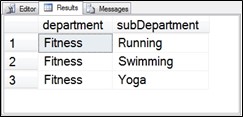
Figure 6.12 Still the same output as both derived tables are turned into CTEs.

With a small query like this the value of cleaning up isn’t always apparent. Consider if each of the CTEs in this example were 15 lines of code, and consider if they were each referenced three or more times. If this were the case the CTE version of the query would be significantly smaller than the derived table version, and would be less likely to have errors since there wouldn’t be duplicated code.

Keep in mind that the idea of converting a derived table into a CTE is just a tool that is available. There is no steadfast rule that says it must be done, and there are probably many examples where the derived table will actually be cleaner code. Use common sense to decide when it is right to convert derived table queries into multiple CTEs.

Theoretical Example

There is the age-old story of the chicken and the egg. Which came first? How could you have a chicken without an egg, but how could you have an egg without a chicken? Such a conundrum! It is one of those questions that has boggled philosophers for more than a thousand years, possibly even longer.

Using databases in software development you could rephrase it as “which came first, the software or the performance problems”? Without the software, there would never be any performance problems, but without the database with the performance problems, the software wouldn’t work!

Often times in a software development environment, applications are built using a test database that is empty, or almost empty. Once the application is moved into a production environment, the size of the tables grows dramatically. Once the tables grow in size the performance of the application usually degrades.

Take the example of the next social networking site. The users table is designed, and the application is built using that table. Even if everyone on the development team adds their own test data on a daily basis, it is unlikely that the users table will end up with more than a thousand rows of data. The social networking site runs great in all of the test scenarios with the data that is available, then it finally launches. The social networking site gets thousands of users, then hundreds of thousands of users, and is headed towards a million users. It grows virally like the social networking dream site.

The problem is that as soon as it grows it starts to experience performance issues that were never considered prior to launch. The problem was the testers never tested the system with very much data in any of the tables. Due to the user interface and sign up process it was difficult to get more than a thousand users in the test database.

As the site grows towards a million users, the investors are getting really excited, an IPO is discussed, and everyone is ready to make more money than they have ever made before. Then it all grinds to a crawl. The login process takes 10 seconds, and then people start to notice that it is taking 30 seconds. Next the login process takes a minute, and people start giving up on the social networking site. The user base drops from almost a million to a hundred thousand, then it drops even further, and suddenly nobody is using the site. At this point the IPO is cancelled, the layoffs begin, and everyone in the company is looking for a new job.

The previous story is completely made up, but it could happen. How would it feel to be the DBA on that project, or even the developer working on the database, how would that look on a resume?

“Destroyed the entire company dream due to lack of planning on the database. Helped with the layoffs after building an architecture that didn’t scale well.”

It would not look so good on any resume.

Here is what could be done to flush out the performance problems with growth. When working in a test environment, plan for growth and add 10 times the expected growth into the test tables. If we are planning for a million users, add 10 million rows into the test table. But how do we do that?

One way this has been done in the past is to create one insert statement, and run it 10,000,000 times. Yes, that will fill up the table, but it won’t be very realistic data. Every row will be exactly the same.

To start with, we will need a table called Users that contains a few columns, and has a couple indexes, one clustered and one not.

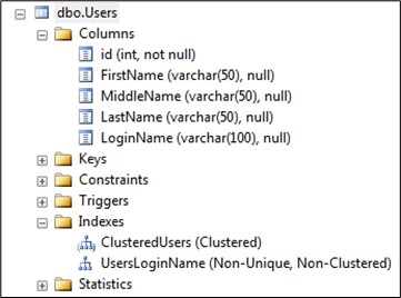
Figure 6.13 Users table, to fill with test data.

We could fill it by doing the following:

INSERT INTO [dbo].[Users]
([FirstName], [MiddleName], [LastName], [LoginName])
VALUES
(‘Steve’, ‘Tester’, ‘Stedman’, ‘SteveTesterStedman’);
GO 10000000

Using the GO statement followed by a number tells Management Studio to run the script that number of times. The GO 10000000 means to run the script 10,000,000 times which will put 10 million rows into the Users table. The problem with this method is that every row in the Users table will be exactly the same, and indexing on the LoginName where all the rows are identical won’t give realistic indexing performance.

An alternative is to use a CTE. First create the CTE to generate the data, and then use it with an INSERT statement. Let’s start with the query that we used earlier in the chapter and we will add in another CTE for middle names. The query layout and new line characters have been adjusted from the previous query and the middle names have been added:

;WITH Fnames (Name) AS
(SELECT ‘John’ UNION SELECT ‘Mary’ UNION SELECT ‘Bill’),

Mnames (Name) AS
(SELECT ‘A’ UNION SELECT ‘Ed’ UNION SELECT ‘Helen’) ,

Lnames (Name) AS
(SELECT ‘Smith’ UNION SELECT ‘Gibb’ UNION SELECT ‘Jones’)

SELECT F.Name AS FirstName, M.Name AS MiddleName,
L.Name AS LastName
FROM Fnames AS F
CROSS JOIN Mnames AS M
CROSS JOIN Lnames AS L;

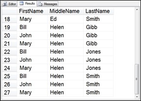
Figure 6.14 First output as we build the CTE to generate users.

Keep in mind that the CROSS JOIN creates the Cartesian product of everything from each of the tables. With three tables cross joined and three rows in each table, this will generate 3 x 3 x 3, or 27 rows. This is nowhere near the 10 million rows that we are looking for, but it is a start.

With this CTE we do get some funny combinations, like Mary Ed Smith. What are the odds that someone named Mary Smith would have the middle name of Ed? Probably very unlikely but it is good test data to fill a table with.

The next step is to add the UserName field to the result set, so we add a fourth CTE as the base value for the user name. When that fourth CTE is accessed we concatenate it with L.Name.

;WITH Fnames (Name) AS
(SELECT ‘John’ UNION SELECT ‘Mary’ UNION SELECT ‘Bill’),

Mnames (Name) AS
(SELECT ‘A’ UNION SELECT ‘Ed’ UNION SELECT ‘Helen’) ,

Lnames (Name) AS
(SELECT ‘Smith’ UNION SELECT ‘Gibb’ UNION SELECT ‘Jones’),

UserNameBase (Name) AS
(SELECT ‘Ace’ UNION SELECT ‘Stallion’ UNION
SELECT ‘Princess’)

SELECT F.Name AS FirstName, M.Name AS MiddleName,
L.Name AS LastName, U.Name + L.Name as UserName
FROM Fnames AS F
CROSS JOIN Mnames AS M
CROSS JOIN Lnames AS L
CROSS JOIN UserNameBase AS U;

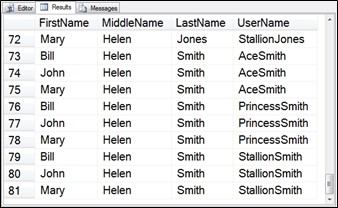
Figure 6.15 CTE output to generate names, and usernames.

Now the total rows generated are 3 x 3 x 3 x3, or 81 rows. Still not the 10 million rows we are looking for, but it’s a start. Next we will add another CTE called Uniqueifier which is intended to help make the username more unique. The outer query references the Uniqueifier CTE twice in the CROSS JOIN and adds it to the front and the back of the value of the UserName field.

;WITH Fnames (Name) AS
(SELECT ‘John’ UNION SELECT ‘Mary’ UNION SELECT ‘Bill’),

Mnames (Name) AS
(SELECT ‘A’ UNION SELECT ‘Ed’ UNION SELECT ‘Helen’) ,

Lnames (Name) AS
(SELECT ‘Smith’ UNION SELECT ‘Gibb’ UNION SELECT ‘Jones’),

UserNameBase (Name) AS
(SELECT ‘Ace’ UNION SELECT ‘Stallion’ UNION
SELECT ‘Princess’),

Uniqueifier(Name) AS
(SELECT ‘A’ UNION SELECT ‘B’ UNION SELECT ‘C’)

SELECT F.Name AS FirstName, M.Name AS MiddleName,
L.Name AS LastName,
Uniq.Name + U.Name + L.Name + Uniq2.Name as UserName
FROM Fnames AS F
CROSS JOIN Mnames AS M
CROSS JOIN Lnames AS L
CROSS JOIN UserNameBase AS U
CROSS JOIN Uniqueifier AS Uniq
CROSS JOIN Uniqueifier AS Uniq2;

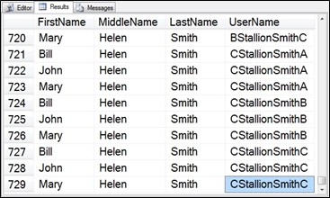
Figure 6.16 CTE output to generate names, and user names with the Uniqueifier CTE added.

Now we get 3 x 3 x 3 x 3 x 3 x 3, or 729 results. Closer, but still not the 10 million rows we want.

Next we add the INSERT INTO statement into the outer query so the output from the CTEs goes into the Users table.

;WITH Fnames (Name) AS
(SELECT ‘John’ UNION SELECT ‘Mary’ UNION SELECT ‘Bill’),

Mnames (Name) AS
(SELECT ‘A’ UNION SELECT ‘Ed’ UNION SELECT ‘Helen’) ,

Lnames (Name) AS
(SELECT ‘Smith’ UNION SELECT ‘Gibb’ UNION SELECT ‘Jones’),

UserNameBase (Name) AS
(SELECT ‘Ace’ UNION SELECT ‘Stallion’ UNION
SELECT ‘Princess’),

Uniqueifier(Name) AS
(SELECT ‘A’ UNION SELECT ‘B’ UNION SELECT ‘C’)

INSERT INTO [dbo].[Users]
           ([FirstName], [MiddleName],
            [LastName], [LoginName])
SELECT F.Name AS FirstName, M.Name AS MiddleName,
       L.Name AS LastName,
       Uniq.Name + U.Name + L.Name + Uniq2.Name as UserName
FROM Fnames AS F
CROSS JOIN Mnames AS M
CROSS JOIN Lnames AS L
CROSS JOIN UserNameBase AS U
CROSS JOIN Uniqueifier AS Uniq
CROSS JOIN Uniqueifier AS Uniq2;

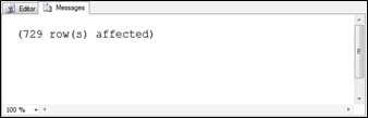
Figure 6.17 CTE output inserting 729 rows into the Users table.

729 rows inserted into the Users table, still not 10 million rows. We can get there fairly easily. Add to the CTEs until we have 15 first names, 15 middle names, 15 user name bases, and 15 Uniqueifier rows. This gives us 15 x 15 x 15 x 15 x 15 x 15, or 11,390,625 rows, just over the 10 million that we are looking for. This will be plenty of user data to simulate a big table.

When the query gets run with 15 names each on the five CTEs, we get the output as shown in Figure 6.18.

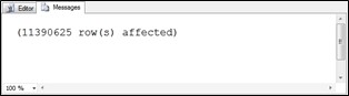
Figure 6.18 Just over 11 million rows inserted into the Users table.

At this point, with a single INSERT INTO statement combined with a SELECT statement it took just a couple minutes to run, we can quickly and easily add millions of rows into a table for testing purposes.

Summary

Multiple CTEs can be used in queries in several ways; independent of each other, building on each other, nested, or a combination. There can be many levels of nesting in CTEs if it makes sense for a specific query.

One of the key things to remember with multiple CTEs is their scope. A CTE is only visible in the current T-SQL statement, and it is only visible after it has been declared. A CTE can reference itself or other CTEs declared before it.

When a CTE references another CTE, this is considered nested. Nesting is a concept of building one CTE upon another. A CTE can reference multiple CTEs in the same statement.

If there are several CTEs being used in a single statement, some of them can be nested, and some can be independent and only accessed from the outer SELECT.

Multiple CTEs in a single statement can be used to quickly populate tables with large amounts of test data. Performance issues can be addressed by testing with large amounts of data in new tables before deploying them into a production system. This type of testing (based on loading up a table with millions of rows from a CTE) could make the difference between success and failure of a database application.

Points to Ponder – Multiple CTEs in a Query

If it made sense to use a CTE to replace a single derived table, it may make sense to use multiple CTEs to replace multiple different derived tables.
A CTE query can reference named CTEs prior to its declaration, but not after. This is considered a nested CTE.
In multiple CTE queries, CTEs can be nested, but it is not required. There could be some nested, and some that are independent.
A common use of multiple CTEs it to generate test data to fill in a table.
Additional CTEs are separated from the previous CTE with a comma.

Review Quiz – Chapter Six

When adding a second CTE into a query where the second CTE references the first CTE is known as:
Recursion
Polymorphism
Nesting
Redundancy
1. When nesting CTEs the depth of nesting is limited to how many levels?
Two levels of nesting.
Sixteen levels of nesting.
100 levels of nesting.
More than should really ever be used.
1. With multiple CTEs in a query the scope of a CTE is (choose the best answer):
A CTE can only be used in a single query.
A CTE can be referenced from anywhere in the current batch.
Only the current CTE and following CTEs in the query can access a CTE.
The scope is limited to a single query, and only the current CTE. Following CTEs in the query and the outer query can access a CTE.

Answer Key

Multiple CTEs in a query that reference earlier CTEs is called nesting. The answer of recursion would be incorrect, because recursion is the term applied to a CTE that references itself. Polymorphism and redundancy don’t apply to CTEs at all. The correct answer is (c).
In SQL Server 2005 the limit to nesting is 256 levels, and In SQL Server 2008 or newer, the limit is based on the amount of memory present. Any query with more than a few dozen CTEs would be very difficult to understand and maintain. The correct answer is (d).
The scope is limited to a single query, and only the current CTE. Following CTEs in the query and the outer query can access a CTE. A CTE is not allowed to be referenced by CTEs declared earlier in the query. The correct answer is (d).